[1]:
from gcpds.utils import loaddb
from matplotlib import pyplot as plt
import numpy as np
from scipy.fftpack import fft, fftfreq, fftshift
from scipy.signal import welch
from datetime import datetime, timedelta

db = loaddb.BCI_CIV_2a('BCI2a_database')
db.load_subject(1)
data, _ = db.get_data()
fs = db.metadata['sampling_rate']
data.shape
[1]:
(273, 22, 1750)
Frequency filters
[2]:
from gcpds.filters import frequency as flt
The input data format use the default trials,channels,time and the value of the sampling frequency in Hertz.
[3]:
print(f"{data.shape} -> (trials,channels,time)")
print(f"{fs} Hz -> Sampling frequency")
(273, 22, 1750) -> (trials,channels,time)
250 Hz -> Sampling frequency
Predefined filters
All predefined filters have the order N=5 (for bandpass) and the quality factor Q=3 (notch).
There are some predefined filters: notch60, band545, band330, band245, band440, band150, band713, band1550 and band550
There is 2 notch filters: notch50 and notch60
[112]:
filtered_data = flt.notch60(data, fs=fs)
data.shape, filtered_data.shape
[112]:
((273, 22, 1750), (273, 22, 1750))
9 EEG common use filters: band545, band330, band245, band440, band150, band713, band1550, band550, band1100
[96]:
flt.band545(data, fs=fs)  # bandpass 5-45 Hz
flt.band1550(data, fs=fs);  # bandpass 15-50 Hz
and 4 EEG waves filters: delta, theta, alpha, beta, mu (an alpha alias).
Filter |
Low frequency |
High frequency |
Order |
|---|---|---|---|
delta |
2 Hz |
5 Hz |
5 |
theta |
5 Hz |
8 Hz |
5 |
alpha, mu |
8 Hz |
12 Hz |
5 |
beta |
13 Hz |
30 Hz |
5 |
[97]:
flt.delta(data, fs=fs)  # bandpass for delta waves
flt.alpha(data, fs=fs);  # bandpass for alpha waves
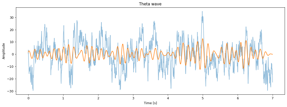
[110]:
plt.figure(figsize=(15, 5), dpi=90)

t = np.arange(data.shape[2]) / fs
plt.plot(t, data[0, 0], alpha=0.5)
plt.plot(t, flt.theta(data, fs=fs)[0, 0])

plt.title('Theta wave')
plt.ylabel('Amplitude')
plt.xlabel('Time [s]')
plt.show()
Recompile predefined filters
In order to change the default order or the quality factor for predefined filters we must re-compile the filters first.
[3]:
flt.compile_filters(N=10, Q=5)
[3]:
flt.band545(data, fs=fs)  # bandpass 5-45 Hz and order N=10
flt.band1550(data, fs=fs)  # bandpass 15-50 Hz and order N=10
flt.notch60(data, fs=fs);  # quality factor Q=5
Custom filters
A custom bandpass, lowpass, hihghpass and notch filter can be defined with GenericButterBand, GenericButterLowPass, GenericButterHighPass and GenericNotch respectively.
[3]:
band880 = flt.GenericButterBand(f0=8, f1=80, N=7)
band880(data, fs=250);

notch55 = flt.GenericNotch(f0=55, Q=5)
notch55(data, fs=250);

low100 = flt.GenericButterLowPass(f0=100, N=5)
low100(data, fs=250);

high100 = flt.GenericButterHighPass(f0=100, N=5)
high100(data, fs=250);
Filters set
In order to apply a set of filters to the same signal, FiltersSet can be defined to reduce the implementation.
[6]:
my_set = flt.FiltersSet(flt.notch60, flt.band545)
my_set(data, fs=250);
Input shape
All filters can work with multidimensional arrays, by default the filter is applied to the index -1, this can be changed with the argument axis.
[12]:
data = np.random.random((10,150,8,100))
flt.notch60(data).shape
[12]:
(10, 150, 8, 100)
[13]:
data = np.random.random((10,150,8,100))
flt.notch60(data, axis=1).shape
[13]:
(10, 150, 8, 100)
Filtering time series
Is possible to use vectors of timestamps, so internally the sampling frequency is calculated, also, is possible to use a vector with the start and the end (in seconds).
[3]:
data = np.random.random(1000)
t = np.linspace(datetime.now().timestamp(), (datetime.now() + timedelta(seconds=15)).timestamp(), 1000)

flt.alpha(data, timestamp=t).shape
[3]:
(1000,)
[6]:
flt.alpha(data, timestamp=[0, 15]).shape # Start and end in seconds
[6]:
(1000,)
About sample frequency
This filtering approach needs the sampling frequency in every call in order to apply the filter, this feature enables to change dynamically between databases with others characteristics.